Lecture 12 - introduction to dynamic programming

Listen To Part 12-1

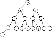
15.1-5 Given an element x in an n-node order-statistic binary tree and a natural number i, how can the ith successor of x be determined in time.  

This problem can be solved if our data structure supports two operations:

• Rank(x) - what is the position of x in the total order of keys?
• Get(i) - what is the key in the ith position of the total order of keys?

What we are interested in is Get(Rank(x)+i).

In an order statistic tree, each node x is labeled with the number of nodes contained in the subtree rooted in x.

Implementing both operations involves keeping track of how many nodes lie to the left of our path.

Listen To Part 12-6

Optimization Problems

In the algorithms we have studied so far, correctness tended to be easier than efficiency. In optimization problems, we are interested in finding a thing which maximizes or minimizes some function.  

In designing algorithms for optimization problem - we must prove that the algorithm in fact gives the best possible solution.

Greedy algorithms, which makes the best local decision at each step, occasionally produce a global optimum - but you need a proof!  

Dynamic Programming

Dynamic Programming is a technique for computing recurrence relations efficiently by sorting partial results.  

Listen To Part 12-9

Computing Fibonacci Numbers

Implementing it as a recursive procedure is easy but slow!  

We keep calculating the same value over and over!

How slow is slow?

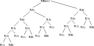
Thus , and since our recursion tree has 0 and 1 as leaves, means we have calls!

Listen To Part 12-10

What about Dynamic Programming?

We can calculate in linear time by storing small values:

  

  

For i=1 to n

		    

Moral: we traded space for time.

Dynamic programming is a technique for efficiently computing recurrences by storing partial results.

Once you understand dynamic programming, it is usually easier to reinvent certain algorithms than try to look them up!

Dynamic programming is best understood by looking at a bunch of different examples.

I have found dynamic programming to be one of the most useful algorithmic techniques in practice:

• Morphing in Computer Graphics
• Data Compression for High Density Bar Codes
• Utilizing Grammatical Constraints for Telephone Keypads

Listen To Part 12-11

Multiplying a Sequence of Matrices

Suppose we want to multiply a long sequence of matrices .  

Multiplying an matrix by a matrix (using the common algorithm) takes multiplications.

We would like to avoid big intermediate matrices, and since matrix multiplication is associative, we can parenthesise however we want.

Matrix multiplication is not communitive, so we cannot permute the order of the matrices without changing the result.

Listen To Part 12-12

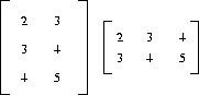
Example

Consider , where A is , B is , C is , and D is .

There are three possible parenthesizations:

The order makes a big difference in real computation. How do we find the best order?

Let M(i,j) be the minimum number of multiplications necessary to compute .

The key observations are

• The outermost parentheses partition the chain of matricies (i,j) at some k.
• The optimal parenthesization order has optimal ordering on either side of k.  

Listen To Part 12-13

A recurrence for this is:

If there are n matrices, there are n+1 dimensions.

A direct recursive implementation of this will be exponential, since there is a lot of duplicated work as in the Fibonacci recurrence.

Divide-and-conquer is seems efficient because there is no overlap, but ...

There are only substrings between 1 and n. Thus it requires only space to store the optimal cost for each of them.

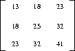
We can represent all the possibilities in a triangle matrix. We can also store the value of k in another triangle matrix to reconstruct to order of the optimal parenthesisation.

The diagonal moves up to the right as the computation progresses. On each element of the kth diagonal |j-i| = k.

For the previous example:

Listen To Part 13-3

Procedure MatrixOrder

for i=1 to n do M[i, j]=0

for diagonal=1 to n-1

		 for i=1 to n-diagonal do

		 		 j=i+diagonal

		 		   

		 		 faster(i,j)=k

return [m(1, n)]

Procedure ShowOrder(i, j)

if (i=j) write (  )

else

		      k=factor(i, j)

		      write ``(''

		     ShowOrder(i, k)

		    write ``*''

		   ShowOrder (k+1, j)

		  write ``)''

Listen To Part 13-4

A dynamic programming solution has three components:

 

1. Formulate the answer as a recurrence relation or recursive algorithm.
2. Show that the number of different instances of your recurrence is bounded by a polynomial.
3. Specify an order of evaluation for the recurrence so you always have what you need.

Listen To Part 13-5

Approximate String Matching

A common task in text editing is string matching - finding all occurrences of a word in a text.     

Unfortunately, many words are mispelled. How can we search for the string closest to the pattern?

Let p be a pattern string and T a text string over the same alphabet.

A k-approximate match between P and T is a substring of T with at most k differences.

Differences may be:

1. the corresponding characters may differ: KAT CAT
2. P is missing a character from T: CAAT CAT
3. T is missing a character from P: CT CAT

Approximate Matching is important in genetics as well as spell checking.

Listen To Part 13-6

A 3-Approximate Match

A match with one of each of three edit operations is:

P = unescessaraly

T = unnecessarily

Finding such a matching seems like a hard problem because we must figure out where you add blanks, but we can solve it with dynamic programming.

D[i, j] = the minimum number of differences between and the segment of T ending at j.

D[i, j] is the minimum of the three possible ways to extend smaller strings:

1. If then D[i-1, j-1] else D[i-1, j-1]+1 (corresponding characters do or do not match)
2. D[i-1, j]+1 (extra character in text - we do not advance the pattern pointer).
3. D[i, j-1]+1 (character in pattern which is not in text).

Once you accept the recurrence it is easy.

To fill each cell, we need only consider three other cells, not O(n) as in other examples. This means we need only store two rows of the table. The total time is O(mn).

Listen To Part 13-10

Boundary conditions for string matching

What should the value of D[0,i] be, corresponding to the cost of matching the first i characters of the text with none of the pattern?  

It depends. Are we doing string matching in the text or substring matching?

• If you want to match all of the pattern against all of the text, this meant that would have to delete the first i characters of the pattern, so D[0,i] = i to pay the cost of the deletions.
• if we want to find the place in the text where the pattern occurs? We do not want to pay more of a cost if the pattern occurs far into the text than near the front, so it is important that starting cost be equal for all positions. In this case, D[0,i] = 0, since we pay no cost for deleting the first i characters of the text.

In both cases, D[i,0] = i, since we cannot excuse deleting the first i characters of the pattern without cost.

Listen To Part 13-9

What do we return?

If we want the cost of comparing all of the pattern against all of the text, such as comparing the spelling of two words, all we are interested in is D[n,m].

But what if we want the cheapest match between the pattern anywhere in the text? Assuming the initialization for substring matching, we seek the cheapest matching of the full pattern ending anywhere in the text. This means the cost equals .

This only gives the cost of the optimal matching. The actual alignment - what got matched, substituted, and deleted - can be reconstructed from the pattern/text and table without an auxiliary storage, once we have identified the cell with the lowest cost.

Listen To Part 13-11

How much space do we need?

 

Do we need to keep all O(mn) cells, since if we evaluate the recurrence filling in the columns of the matrix from left to right, we will never need more than two columns of cells to do what we need. Thus O(m) space is sufficient to evaluate the recurrence without changing the time complexity at all.

Unfortunately, because we won't have the full matrix we cannot reconstruct the alignment, as above.

Saving space in dynamic programming is very important. Since memory on any computer is limited, O(nm) space is more of a bottleneck than O(nm) time.

Fortunately, there is a clever divide-and-conquer algorithm which computes the actual alignment in O(nm) time and O(m) space.