Connected Components

  

 

Input description: A directed or undirected graph G.

Problem description: Traverse each edge and vertex of all connected components of G.

Discussion: The connected components of a graph represent, in grossest terms, the pieces of the graph. Two vertices are in the same component of G if and only if there is some path between them.   

Finding connected components is at the heart of many graph applications. For example, consider the problem of identifying clusters in a set of items.   We can represent each item by a vertex and add an edge between each pair of items that are deemed ``similar.'' The connected components of this graph correspond to different classes of items.

Testing whether a graph is connected is an essential preprocessing step for every graph algorithm.   Such tests can be performed so quickly and easily that you should always verify that your input graph is connected, even when you know it has to be.   Subtle, difficult-to-detect bugs often result when your algorithm is run only on one component of a disconnected graph.

Testing the connectivity of any undirected graph is a job for either depth-first or breadth-first search, as discussed in Section .     Which one you choose doesn't really matter. Both traversals initialize a component-number field for each vertex to 0, and then start the search for component 1 from vertex . As each vertex is visited, the value of this field is set to the current component number. When the initial traversal ends, the component number is incremented, and the search begins again from the first vertex with component-number still 0. Properly implemented using adjacency lists, this runs in O(n+m), or time linear in the number of edges and vertices.

Other notions of connectivity also arise in practice:

• What if my graph is directed? - There are two distinct definitions of connected components for directed graphs. A directed graph is weakly connected if it would be connected by ignoring the direction of edges.   Thus a weakly connected graph consists of a single piece. A directed graph is strongly connected if there is a directed path between every pair of vertices.     This distinction is best made clear by considering a network of one- and two-way streets in a city. The network is strongly connected if it is possible to drive legally between every two positions. The network is weakly connected if it is possible to drive legally or illegally between every two positions. The network is disconnected if there is no possible way to drive from a to b.

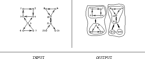
  The weakly and strongly connected components define unique partitions on the vertices. The output figure above illustrates a directed graph consisting of two weakly connected or five strongly connected components (also called blocks of G).

  Testing whether a directed graph is weakly connected can be done easily in linear time. Simply turn all edges into undirected edges and use the DFS-based connected components algorithm described above. Tests for strong connectivity are somewhat more complicated. The simplest algorithm performs a breadth-first search from each vertex and verifies that all vertices have been visited on each search. Thus in O(mn) time, it can be confirmed whether the graph is strongly connected. Further, this algorithm can be modified to extract all strongly connected components if it is not.

  In fact, strongly connected components can be found in linear time using one of two more sophisticated DFS-based algorithms. See the references below for details. It is probably easier to start from an existing implementation below than a textbook description.

• How reliable is my network; i.e. how well connected is it? -     A chain is only as strong as its weakest link.   When it is missing one or more links, it is disconnected.   The notion of connectivity of graphs measures the strength of the graph - how many edges or vertices must be removed in order to break it, or disconnect it. Connectivity is an essential invariant for network design and other structural problems.

  Algorithmic connectivity problems are discussed in Section .   In particular, biconnected components are pieces of the graph that result by cutting the edges incident on a single vertex. All biconnected components can be found in linear time using a DFS-based algorithm. Vertices whose deletion disconnects the graph belong to more than one biconnected component, although edges are uniquely partitioned among them.

• Is the graph a tree? How can I find a cycle if one exists? -     The problem of cycle identification often arises, particularly with respect to directed graphs. For example, testing if a sequence of conditions can deadlock often reduces to cycle detection.   If I am waiting for Fred, and Fred is waiting for Mary, and Mary is waiting for me, we are all deadlocked.

  For undirected graphs, the analogous problem is tree identification. A tree is, by definition, an undirected, connected graph without any cycles. As described above, a depth-first search can be used to test whether it is connected. If the graph is connected and has n-1 edges for n vertices, it is a tree.

  Depth-first search can be used to find cycles in both directed and undirected graphs. Whenever we encounter a back edge in our DFS, i.e. an edge to an ancestor vertex in the DFS tree, the back edge and the tree together define a directed cycle. No other such cycle can exist in a directed graph. Directed graphs without cycles are called DAGs (directed acyclic graphs). Topological sorting (see Section ) is the fundamental operation on DAGs.

Implementations:     LEDA (see Section ) provides good implementations of breadth-first and depth-first search, connected components and strongly connected components, all in C++. XTango (see Section ) is an algorithm animation system   for UNIX and X-windows, which includes an animation of depth-first search.

Pascal implementations of BFS, DFS,   and biconnected and strongly connected components appear in [MS91]. See Section for details. Combinatorica [Ski90] provides Mathematica implementations    of the same routines. See Section .

The Stanford GraphBase (see Section ) contains routines to compute biconnected and strongly connected components.    An expository implementation of BFS and DFS in Fortran appears in [NW78] (see Section ).

Notes:   Depth-first search was first used in algorithms for finding paths out of mazes, and dates back to the nineteenth century [Luc91, Tar95]. Breadth-first search was first reported to find the shortest path out of mazes by Moore in 1957 [Moo59].

Hopcroft and Tarjan [HT73b, Tar72] first established depth-first search as a fundamental technique for efficient graph algorithms. Expositions on depth-first and breadth-first search appear in every book discussing graph algorithms, with [CLR90] perhaps the most thorough description available.

The first linear-time algorithm for strongly connected components is due to Tarjan [Tar72], with expositions including [Baa88, Eve79a, Man89]. Another algorithm, simpler to program and slicker, to find strongly connected components is due to Sharir and Kosaraju. Good expositions of this algorithm appear in [AHU83, CLR90].

Related Problems: Edge-vertex connectivity (see page ), shortest path (see page ).